Mastering Logistic Regression in Excel: A 6 Step How-To Guide

Learning how to do logistic regression in Excel can add a powerful predictive tool to your toolbox. With artificial intelligence and machine learning dominating the technology main stage, logistic regression and other predictive algorithms like linear regression have begun to permeate mainstream business vernacular. Because logistic regression can predict the likelihood of an event, it has a wide range of business applications, from fraud detection to sales revenue forecasting.

Predictive algorithms have long been accessible in spreadsheet applications like Excel, though they lack the compute, storage, and processing capabilities of the cloud and big data infrastructure. We’ll show you how to use them to do a logistic regression in Excel in six steps, giving you the ability to make predictions from your data right on your desktop.

How to do a Logistic Regression in Excel

Logistic regression is a statistical analysis technique for transforming a linear function’s output into a probability value. Unlike linear regression, which predicts continuous outcomes, logistic regression predicts the probability of an event occurring by using a logistic function to predict the probability of a binary outcome. These types of predictions that categorize based on two outcomes are called binary classification tasks.

For our example, you’ll perform a logistic regression in Excel to determine whether a college basketball player is likely to get drafted into the NBA. Your dataset includes basic performance metrics from the previous season:

• Average points
• Rebounds
• Assists

Because logistic regression is a binary classification problem, the target prediction is a simple binary classification value of the likelihood of being drafted:

• 0 = no
• 1 = yes

Step 1: Insert Historical Data and Regression Coefficients

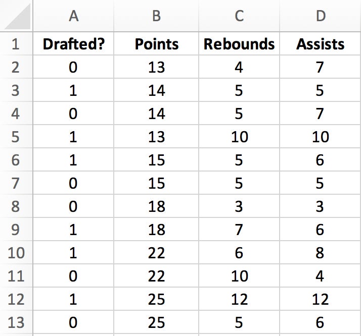
The first step is to create the tabular structure in Excel for holding your dataset and performing calculations and transformations.

1. In a new Excel sheet, create four columns labeled ““Points,” “Rebounds,” “Assists,” and “Drafted?”
2. Insert the dataset from the table below.

Once you’ve inserted the dataset, your spreadsheet should look like Figure 1.

Step 2: Create Corresponding Cells for Variables

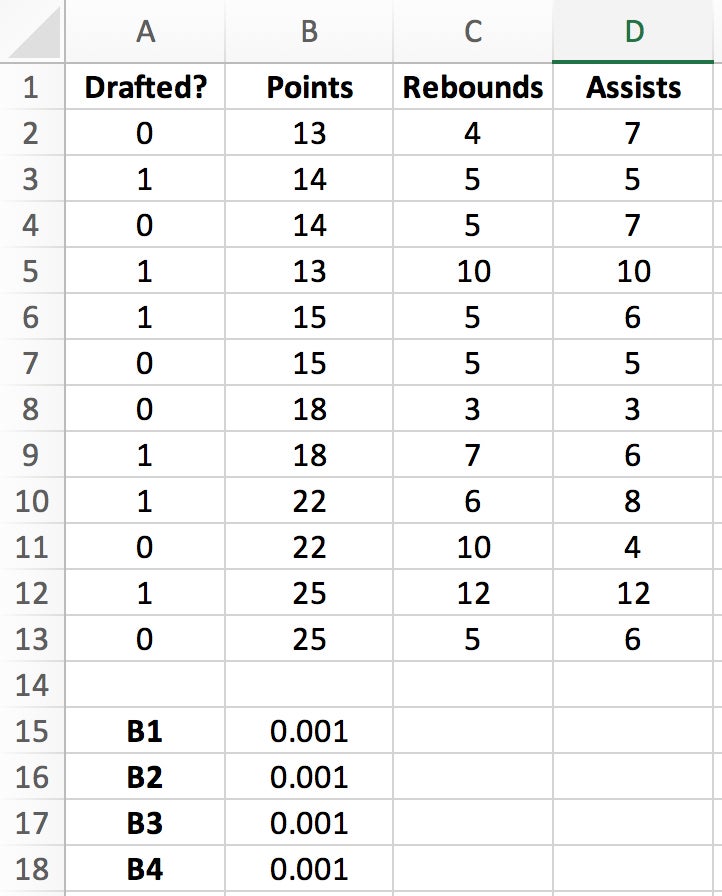
Create a corresponding cell for each of your columnar variables—Points, Rebounds, Assists—to hold your regression coefficients.

1. Skipping a row after the dataset, create three subsequent cells labeled B1, B2, and B3.
2. On the next row, create a cell for the logistic regression’s intercept.
3. Set all four of these values to 0.001 for now; we’ll optimize them in a later step.

Step 3: Create Columns for Coefficient Optimizations

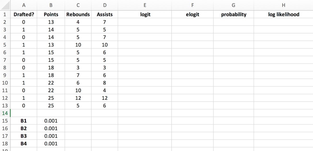
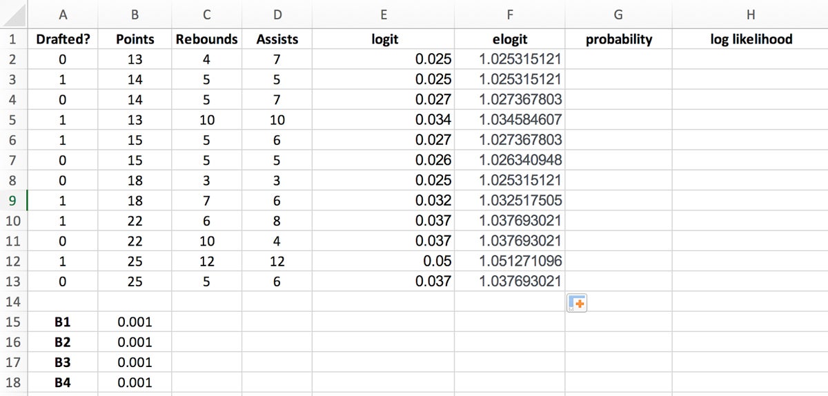
Next we’ll create columns for optimizing the regression coefficients. We’ll need these to calculate predictions in later steps, but for now we’ll focus on populating four new columns:

• Logit: The logarithm of the odds of the probability p of a player getting drafted.
• E^logit: The inverse transformation of logit.
• Probability: The probability of being drafted, expressed as a real number.
• Log Likelihood: Goodness of fit, expressed as a negative number—the closer to zero, the better.

1. Beginning in the first empty column to the right of the dataset, label the four subsequent columns as follows: “logit,” “elogit,” “probability,” and “log likelihood.”

2. Calculate logit values by taking the logarithm of the odds of the probability (p) of a certain event occurring:

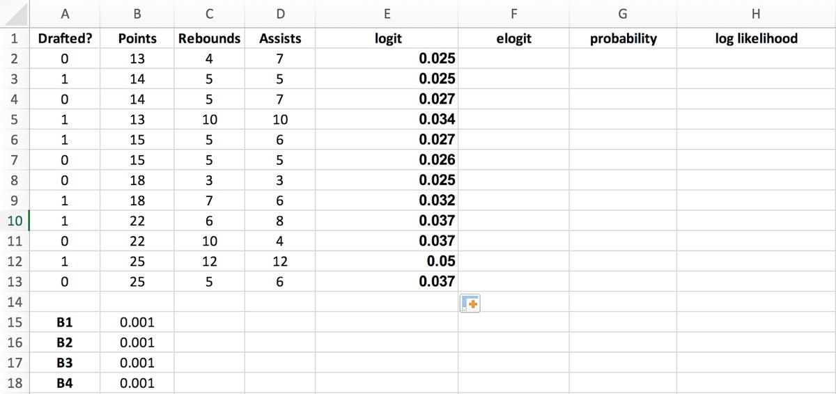
In Excel, you can use the formula $B$15+$B$16*B2+$B$17*C2+$B$18*D2 to easily derive the logit value. Place this formula into the first logit cell and drag the bottom right corner of the highlighted cell to the last logit cell to populate the column.

3. Create e^logit values by returning the result of the constant (e), which is the base of the natural logarithm raised to the power of the value in the logit column. In this example, the base of the natural logarithm comes out to about 2.718.

You can use Excel’s EXP function to get this value. Place the formula =EXP(E2) into the first elogit cell and drag the bottom right corner of the highlighted cell to the last elogit cell to populate the column.

4. Calculate probability values using the following formula for calculating probability (p):

In our example:

• p is the probability of a 1 value (the proportion of 1s, the mean of Y)
• e is the constant with the value ~2.718
• a and b are the parameters of the algorithm

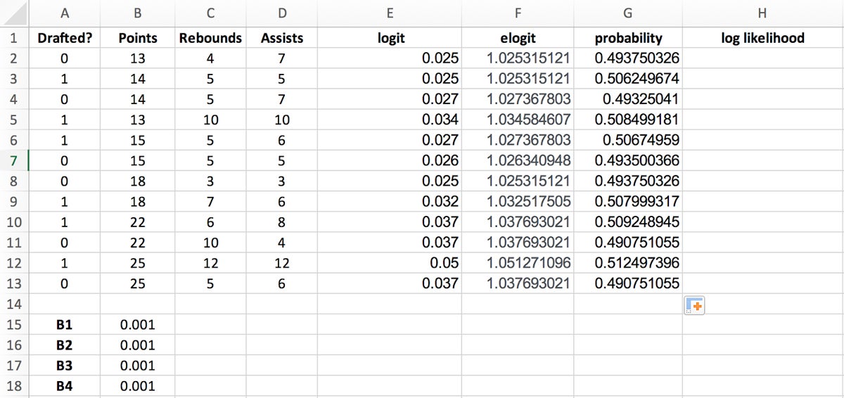
In Excel, you can use the formula =IF(A2=1, F2/(1+F2), 1-(F2/(1+F2))) to derive the probability values by placing this formula into the first probability cell and dragging the bottom right corner of the highlighted cell to the last probability cell to populate the column.

Your spreadsheet should now look like Figure 6.

Step 4: Create and Sum Log Likelihood Values

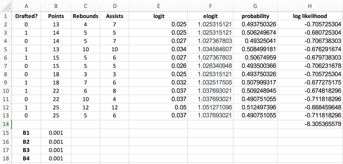
Because adding logarithms is computationally more efficient than multiplying probabilities directly, you’ll need to calculate the log likelihood values to simplify your calculations and make them more practical.

Log likelihood values are calculated by using the following formula:

Log likelihood = LN(probability)

1. Use the formula =LN(G2) to easily derive the log likelihood values in Excel by placing this formula into the first log likelihood cell and dragging the bottom right corner of the highlighted cell to the last log likelihood cell to populate the column.

2. Sum up all the log likelihood values in order to derive the number to maximize to solve for the regression coefficients. You do this easily by placing the formula =SUM(H2:H13) in the cell below the last log likelihood cell.

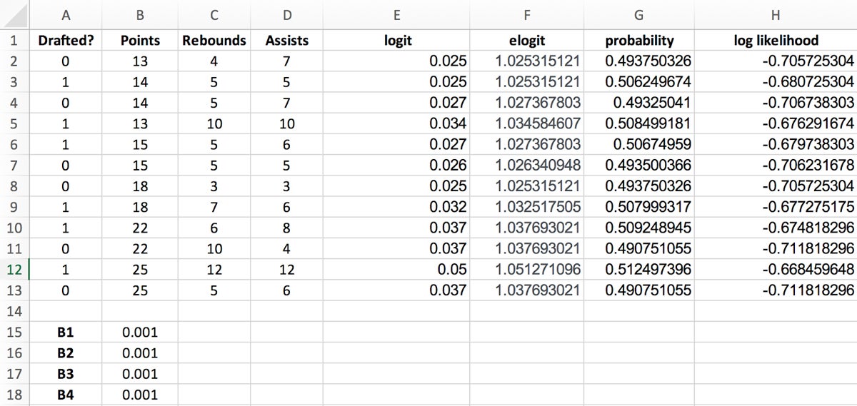
Your spreadsheet should now look like the example in Figure 8.

Step 5: Solve For Regression Coefficients

The last step involves using Excel’s Solver add-in to automatically calculate the regression coefficient estimates.

1. Install Excel’s Solver add-in by clicking first on the Home menu and then the Add-Ins menu.
2. Search for and install Solver by following the prompts.
3. Select the Data menu from the top-level navigation and click Solver on the right-hand side to run the add-in.
4. In the Solver Parameters pane, insert the following values:

• Set Objective: select cell H14 with the sum of the log likelihoods
• To: Max
• By Changing Variable Cells: Select cells B15:B18 containing your regression coefficients
• Make Unconstrained Variables Non-Negative: Uncheck
• Select a Solving Method: GRG Nonlinear

1. Click the “Solve” button.

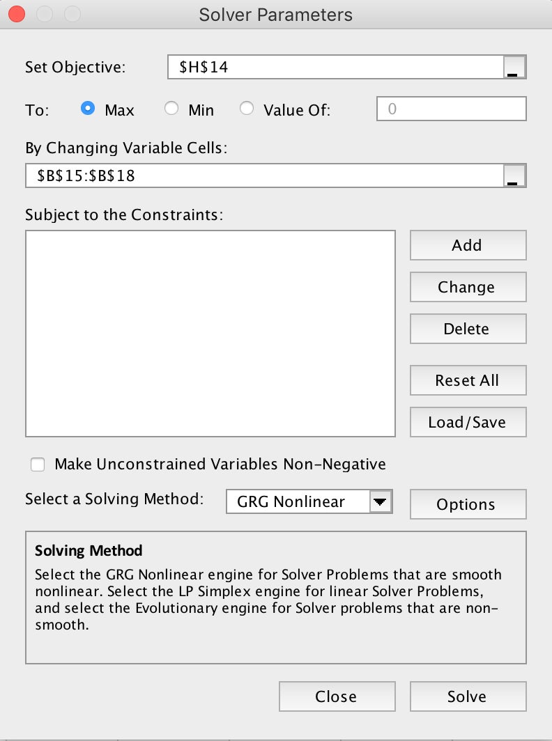
After Solver finishes automatically calculating your regression coefficient estimates, your spreadsheet should look like Figure 10.

The current regression coefficients default to determining the probability of a non-draft:

Draft? = 0

To get the probability of being drafted (Draft? = 1), simply reverse the regression coefficients signs—for example, reverse the -4.643753  in the p(x=0) column for a positive 4.643753 value in the p(x=1) column.

Step 6: Add New Data For New Prediction

Now that you have your regression coefficient estimates, you can plug them into the probability equation to find out whether a new player will get drafted. For this example, let’s say the new player averages 15 points per game, 4 rebounds per game, and 6 assists per game. Again, the formula for calculating the probability of being drafted is:

In this example, the formula would look like the following:

Evaluating this equation yields 0.66, or a 66 percent probability this new player will get drafted.

1. To calculate this in Excel, add the new player’s data to your Excel spreadsheet in a new row to calculate their probability of getting drafted.

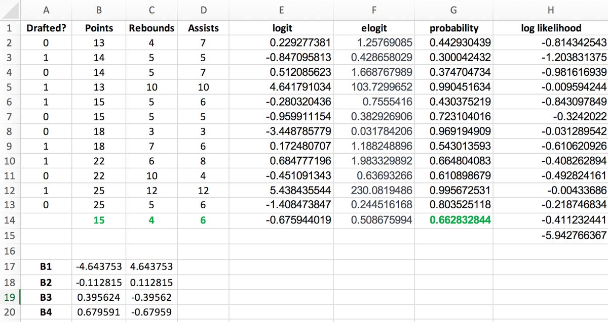
As you can see, the probability of the new player being drafted is also 66 percent, which lines up with the previous manual calculation.

How Does Logistic Regression Work?

Logistic regression involves predicting the probability of a binary event occurring—for example, success/failure, yes/no, churn/no churn). By definition, probability is a measure of the likelihood of an event occurring, ranging from 0 (impossible) to 1 (certain).

Odds, on the other hand, express the likelihood of success compared to the likelihood of failure. For example, if the probability of success is 0.8, the odds of success are 0.8 / (1 – 0.8) = 4. This means there are four times as many favorable outcomes as unfavorable ones.

Log Odds and the Sigmoid Function

Log odds ratio is a calculation method for transforming these odds into a more workable range of values. Specifically, the logistic regression model uses the sigmoid function—denoted as σ(z)—to calculate the log odds ratio, or the logarithm of the odds of success. Mathematically, log odds ratio is represented as:

In this formula, p is the th. By taking the logarithm of the probability’s value, you can map the odds from a scale of 0 to positive infinity, down to a range that extends from negative infinity to positive infinity. In other words, the log odds ratio measures the likelihood of an event happening in one group compared to another, with positive values indicating a higher likelihood in the first group and negative values indicating a higher likelihood in the second group.

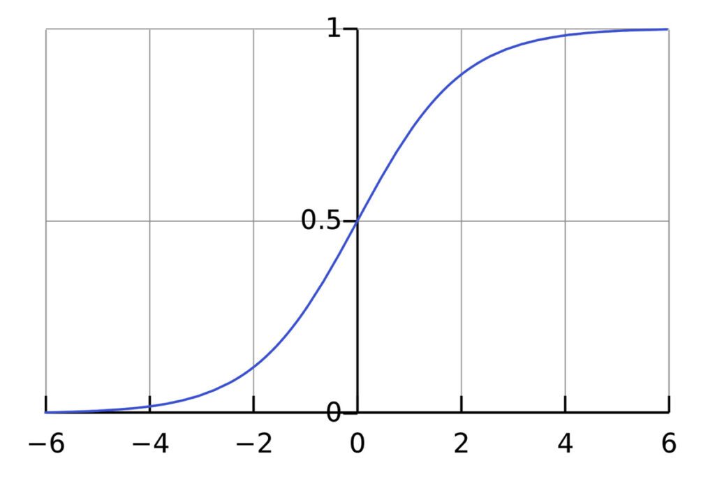
When plotted out on a graph, the output of a logistic regression takes on the shape of a sigmoid (S-shaped) curve.

Interpreting Log Odds Ratio

A logistic regression calculates the log odds ratio for each independent variable. As mentioned earlier, when you see a positive coefficient, it means that as the associated independent variable increases, the log odds of the event increase; subsequently, the probability of the event occurring goes up. Conversely, a negative coefficient suggests that as the variable increases, the log odds (and probability) of the event decrease. By mapping the resulting value to the range—0 or 1]—you can make predictions based on calculating probabilities.

Frequently Asked Questions (FAQs)

What is the difference between linear regression and logistic regression?

Linear regression is used for predicting continuous outcomes, while logistic regression is used for predicting binary outcomes (i.e., the dependent variable is categorical with two possible outcomes).

How can I interpret the odds ratio in logistic regression?

The odds ratio represents the factor by which the odds of the event increase (or decrease) for a one-unit change in the independent variable. If the odds ratio is greater than one, it suggests an increase in the odds of the event. If it’s less than one, it indicates a decrease.

Can logistic regression handle more than two categories in the dependent variable?

No, logistic regression is specifically designed for binary classification problems where the dependent variable has only two categories.

How do I deal with multicollinearity in logistic regression?

Multicollinearity, or scenarios where independent variables are highly correlated, can impact the stability and interpretability of a logistic regression model. Excel’s Data Analysis ToolPak provides a Variance Inflation Factor (VIF) option, which can help identify multicollinearity.

What steps can I take if my logistic regression model doesn’t perform well?

If your model doesn’t perform as expected, you can experiment with different sets of independent variables, address multicollinearity, and explore data transformations.

Bottom Line: Logistic Regressions In Excel Are Beneficial

Whether you’re predicting customer churn, analyzing marketing campaigns, or assessing operational risk factors, logistic regression provides a robust yet elegant framework for predictive modeling and data-driven optimization. The powerful, widely utilized statistical method is a go-to for binary classification problems and is renowned for its interpretability and flexibility in handling various data types; these attributes and more make it a frequently used tool in the data scientist and professional’s statistical toolbox.

If you’re interested in statistical analysis using Excel, learn how to use the spreadsheet tool for Linear Regressions or Monte Carlo Simulations.