How to Use Lists in Excel

Datamation content and product recommendations are editorially independent. We may make money when you click on links to our partners. Learn More.

While a database is generally the smart way to keep track of complex data, sometimes your needs are much simpler. In situations where your data is more like a list or table, Excel has an excellent list management tool designed for the task.

Working on lists in Excel offers advantages over using a database application in that you can see your data very clearly, and you still have all the familiar Excel tools for working with the information. In this Exploring Office 2007 article we’ll take a look at how lists work in both Excel 2007 as well as the older Excel 2003 release.

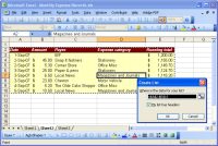
Use the Data > List option to convert data in a worksheet into an Excel 2003 list

» Lists in Excel 2003

Featured Database Solutions

Excel List Function

List management tasks received a boost with the new List tool in Excel 2003. Using this tool you can define an area of a worksheet as a list, which gives the area special properties such as an insert row that you can click to insert a new data row into the list.

In addition, you can position lists side-by-side in the same worksheet, and they act independently of each other. This lets you add or delete a row in one list and the other list will remain unaffected by the changes.

Lists in Excel 2003 also have automatic totals built into them so that you can select the calculation to apply to a list column and Excel will automatically create the formula for you.

See for yourself how easy it is to work with lists in Excel 2003. Open a worksheet containing a table of data. Click somewhere inside the data area and choose Data > List > Create List. Excel makes a guess as to the range containing the data and gives you the option of specifying whether or not your list has headers.

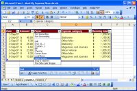
By default Excel lists have the Filter option enabled although this can be disabled, if desired

Select OK if the data in the Create List dialog is correct; otherwise, make your changes and click OK. If your list doesn’t have column headers, deselect the checkbox. Excel will create column headers automatically for you and name them Column1, Column2, etc.

Your list will appear on the screen bounded with a blue line, and it will have the Filter option enabled so that filter arrows appear to the right of each column heading. From these dropdown lists you can select an element with which to filter or sort the column. To undo the filter, choose Data > Filter > Show All.

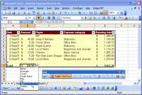
To create totals for the columns in your list, click the Toggle Total Row icon on the List toolbar. Click in the cell below the target column (the one you want the calculation to affect), and a small arrow will appear to its immediate right. Click this arrow and select the calculation you want from the drop-down list that appears.

Microsoft Excel Lists - Subtotal Function

Excel creates calculations for data in your list columns using the Subtotal function

The calculation options include: Average, Count, Count Numbers, Max, Min, Sum, StdDev, or Var. Excel will create a formula for that calculation and show the results for only the visible values in the list. This is because Excel creates its formulas using the Subtotal function so the results reflect only visible cells in the column and not all the cells in it.

An additional benefit of using the List tool in Excel 2003 is that if you create a chart based on the data in the list, and if you later add data to the list, the chart expands automatically to display the new data. Prior to Excel 2003, to create a chart that would expand when additional data was added to a list was extremely difficult, requiring a complex workaround solution.

You can add and delete rows from your list by right clicking and choose Insert > Row or Delete > Row. To add a column to your list, simply type a value into the empty column to the right of the list, and the list expands automatically to include the new column.

If at any time you no longer want to use the List functions in Excel 2003, you can disable this functionality. To do so, click inside the List to activate it and then from the List toolbar click List > Convert to Range and click Yes when prompted to do so. The List will convert back to regular data in an Excel worksheet.

Lists and Tables in Excel 2007

In Excel 2007 tables have replaced lists. Their effect is similar but the process of creating them is a little different. To format a list as a table, select it and from the Home tab select the Format as Table option in the Stylesgroup. Select a table style to apply to your data.

If you have a large table, when you scroll beyond the first screen, you will notice that the column letters A, B, C, D, etc. change to display the table headings. This ensures that you can easily identify the data you are looking at without having to resort to using the Freeze Panes command even when your worksheet is very large.

You manage the heading feature by using Table Tools > Design > Header Row. If the Header Row is enabled, the first row will be formatted differently and appear as column headings; if it’s not, the regular column letters appear.

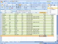
Microsoft Excel 2007 Lists - AutoSum Option

In Excel 2007 you can select an automatic calculation from the AutoSum option on the Home tab

The AutoFilter is enabled by default for all Excel tables, but you can disable this if you like, by selecting the Home button and dropdown the Sort and Filter list and deselect the Filter. The column headings continue to work even if filtering is disabled.

If you select the cell below a column of numbers or text in the table you can click the down-pointing arrow to the right of the AutoSum function on the Home tab’s Editing area. From here you can select a calculation to apply to that column of values.

When you do, the calculation works as a Subtotal function so it adjusts to show the result for all visible cells and not all cells in the table column.

In Excel 2007 you have more attractive table formats than you’ll be used to using in Excel 2003, but apart from these the lists function very much the same in Excel 2007 as in Excel 2003.

Whether you’re working with Lists in Excel 2003 or Tables in Excel 2007, you will find the tools that Excel provides for managing data in a table-like format make Excel a viable alternative to using a database application.

This article was first published on WinPlanet.